
Public PhD Defense
This post contains the content of my PhD defense, together with some extra information and (personal) ideas for further work.
Uncertainty is a fundamental notion, both in our daily lives and in science. Sadly, whereas it was or prime importance on statistics, it has become a secondary notion in current-day computational data science. Conformal prediction tries to fix this issue.
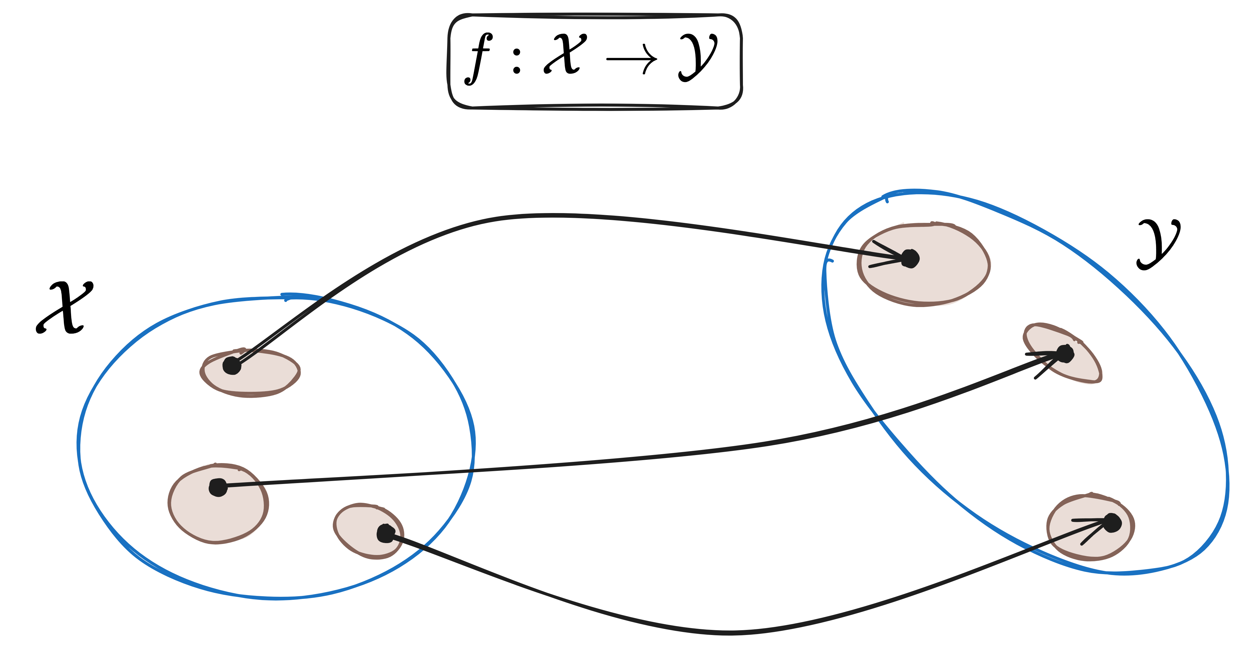
However, before introducing the concept of conformal prediction. Let us take a step back and reconsider what we mean by ‘uncertainty’.1 An ordinary model, which is mathematically simply a function from an input space $\mathcal{X}$ to an output space $\mathcal{Y}$, can be represented as follows.
However, this would mean that our models and mental representation are crisp, i.e. completely accurate and deterministic. In practice, there is often a lot of uncertainty about the data — be it epistemic, i.e. related to a proper lack of knowledge, or aleatoric, i.e. related to inherent stochasticity in the underlying process — and this uncertainty makes it impossible to obtain crisp predictive models as shown below.
However, for our needs, focus will be restricted to those models that assume crisp inputs and produce probability distributions regarding the outputs (conditional on the input).
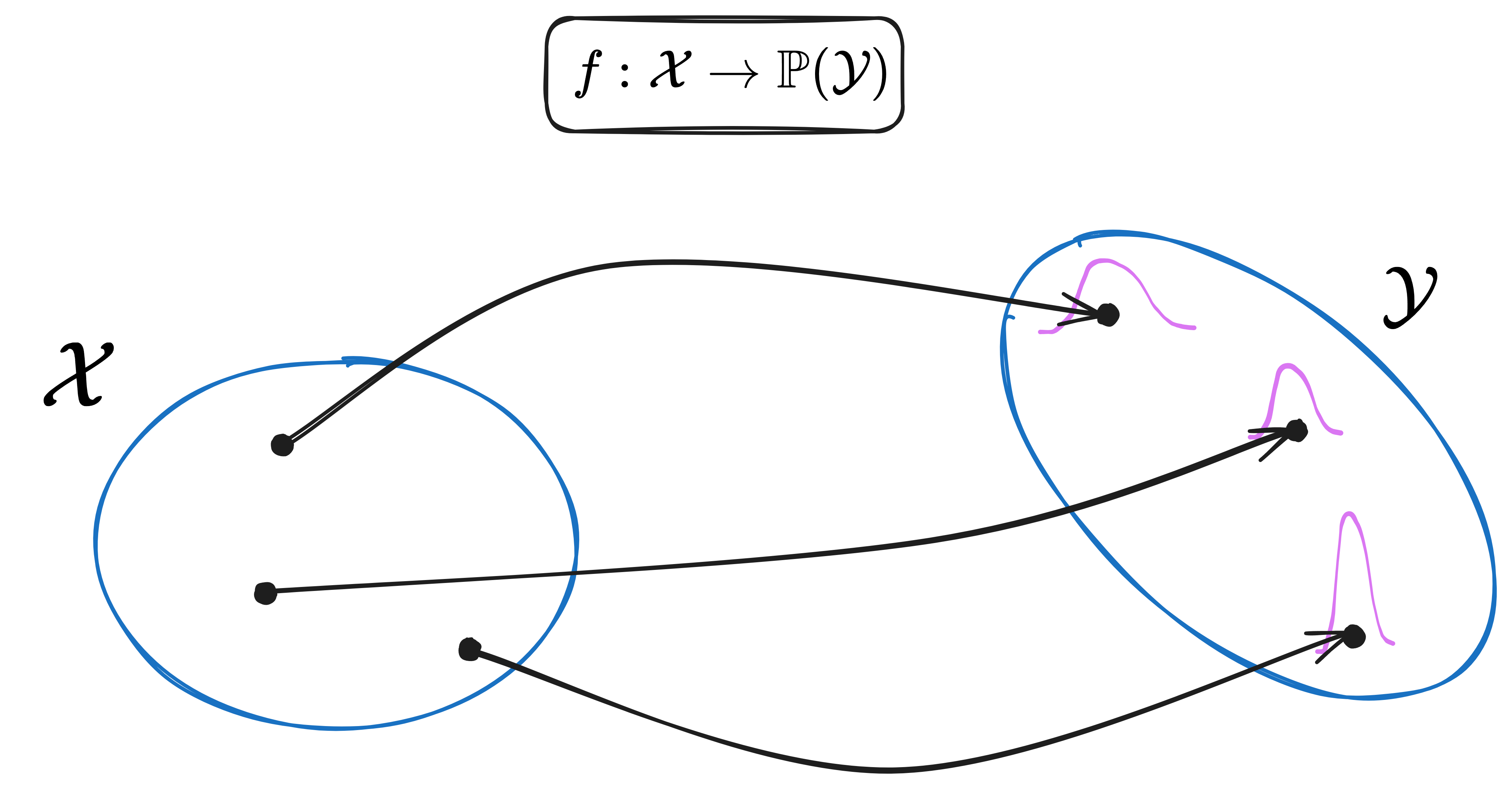
In fact, our focus will be even more restricted. We will only look at models that take crisp inputs and produce sets of possible outputs.
As already mentioned in this previous post on prediction intervals, several methods exist for the construction of confidence predictors: e.g. Bayesian methods and ensemble methods. The reason to focus on methods that produce prediction regions instead of full-fledged probability distributions, is that the former are easier to construct and apply, although the latter contain more information.
A short example might help to clarify this notion. Here, we show two images of numbers and the output of some pretrained confidence predictor.
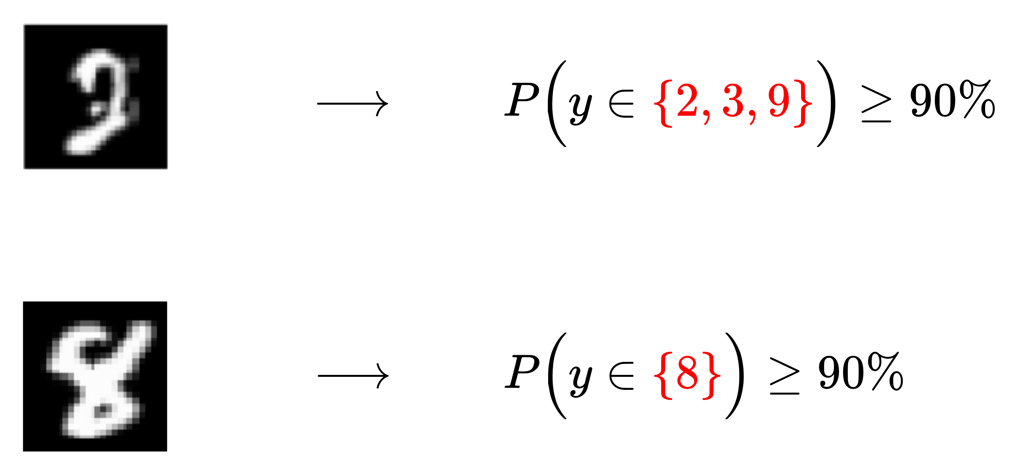
The first image is, at least to me, rather hard to decipher. Consequently, a reasonable confidence predictor would output a set containing multiple possibilities (here: 2, 3 and 9) that cover the true number with high probability ($90\%$ in this case). The second image, on the other hand, is sharper and, as such, our model outputs a set with a single (correct) number.
The purpose of this post will be to delve into more detail about the statement “cover the true number with high probability”. What do we mean with high probability? Is this over all possible data points? Is this conditional on the true number? Many possibilities exist.
Many standard techniques from statistics have important limitations that make them unappealing to machine learning practitioners. Three main classes are:
- Model limitations (e.g. linearity),
- Data assumptions (e.g. ordinal data or normality), and
- Computational (in)efficiency (e.g. Bayesian inference).
Luckily, there exists an alternative: ‘Conformal Prediction’. This has
- No model constraints,
- Weak data assumptions,
- Efficient implementations, and
- Can incorporate modern methodologies (e.g. online learning).
Item 1 can be taken literally, all measurable functions are allowed. For Item 2, the correct assumption is the following one.2
A nice example here is Polya’s urn (see the image below). If you have a bag of marbles with two colours, let’s say green and red, the probability of drawing a given colour changes throughout sequential draws (since the number of marbles changes), but the joint of probabilities do not depend on the order.
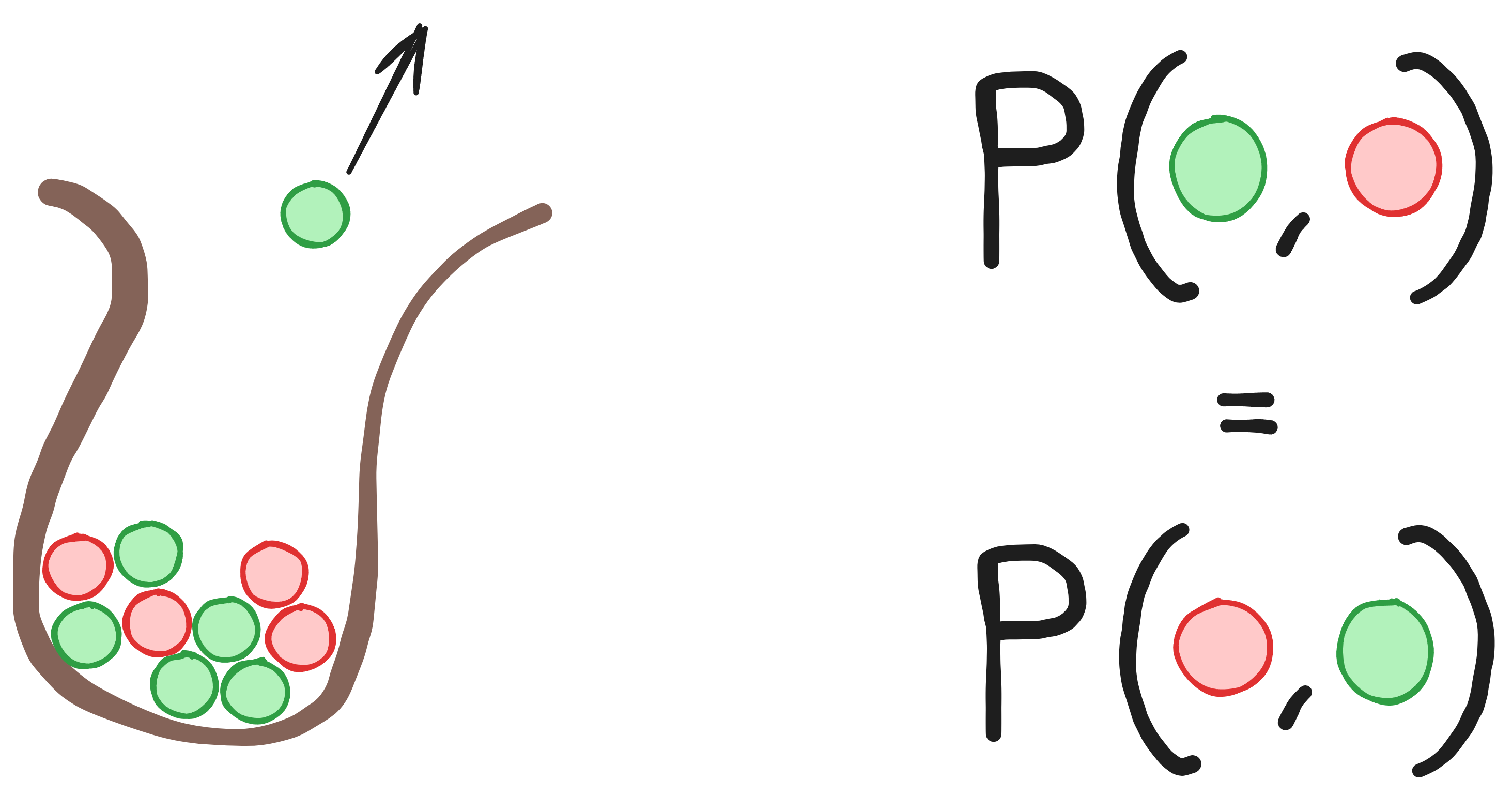
The general idea behind conformal prediction is that exchangeability, i.e. the irrelevant order of data points, implies that the rank of data points, when using ordinal data, is uniformly distributed. This apparently innocuous fact is the working horse of my thesis.
However, not all kinds of data are ordinal. To this end, one needs a way to convert data points into, preferably, numbers.
Try and see if you can find out which nonconformity measure was used in the example below (or read on to find out about it).
\begin{array}{cccc}
\hline
x&\rho(x)&y&A(x,y) \\
\hline
0.5&1&2.5&1.5 \\
2.5&5&3&2 \\
1&2&10&8 \\
\hline
\end{array}
Typical nonconformity measures in the one-dimensional regression setting are (denote the regressor by $\rho:\mathcal{X}\rightarrow\mathbb{R}$):
- Standard (residual) score
- Normalized (residual) score
where $\sigma:\mathcal{X}\rightarrow\mathbb{R}^+_0$ is an uncertainty estimate such as the standard deviation.
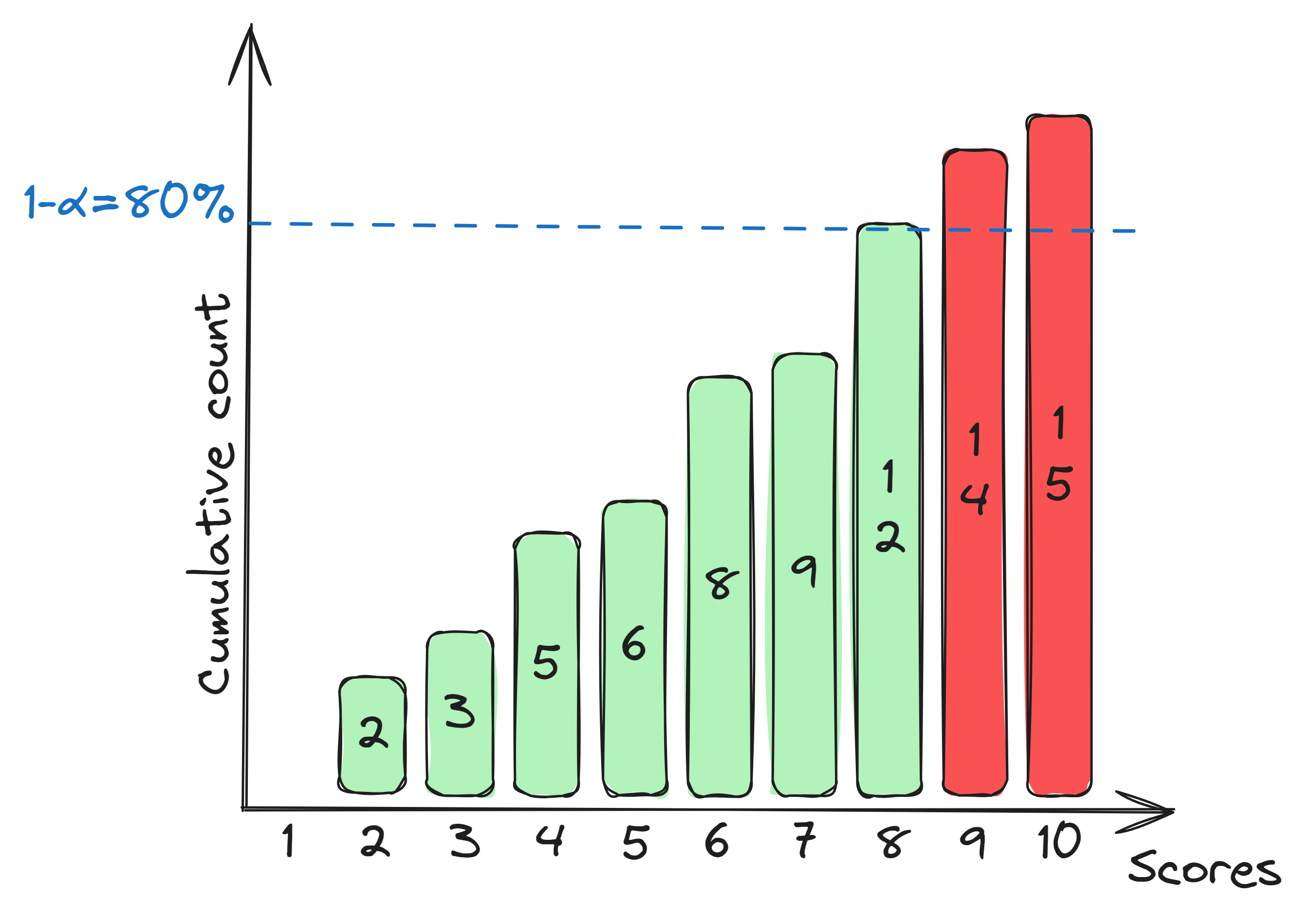
The (inductive) conformal prediction algorithm has the following simple workflow:
- Choose a calibration set ${(x_i,y_i)}_{i\leq n}$, a nonconformity measure $A:\mathcal{X}\times\mathcal{Y}\rightarrow\mathbb{R}$ and a significance level $\alpha\in[0,1]$.
- Calculate the score $a_i:=A(x_i,y_i)$ for every calibration point.
- Determine the critical score $a^*:=q_{(1-\alpha)\left(1 + 1/n\right)}\bigl(\{a_i\}_{i\leq n}\bigr)$.
- For a new $x\in\mathcal{X}$, include all $y\in\mathcal{Y}$ such that $A(x,y)\leq a^*$.
The corresponding pseudocode (in Python, using the PyTorch library) is shown below:
   def conformalize(model, X, y, alpha, inflate = True):
        scores = model.predict(X, y)
        scores, _ = torch.sort(scores)
        level = min((1 + ((1 / scores.shape[0]) if inflate else 0)) * (1 - alpha), 1)
        index = math.ceil(level * scores.shape[0]) - 1
        return scores[index].item()
Although the necessary code to perform (inductive) conformal prediction is remarkably short, this procedure’s true power lies in the strong guarantees that come with it (for free)!
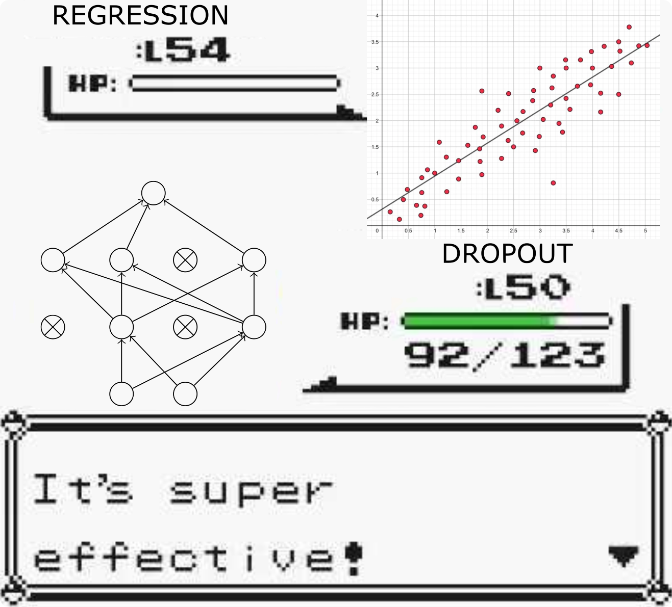
One of my favourite baseline models for uncertainty quantification (before applying conformal prediction) is the mean-variance ensemble. In particular, the dropout-based mean-variance ensemble. A mean-variance estimator is a model, beit classical or deep learning-based, that not only gives a point prediction (in this case the mean), but at the same time also predicts the standard deviation or variance of the target conditional distribution. Dropout, on the other hand, is a popular regularization technique in deep learning where random neurons turned off during training. By extending this behaviour to test time, we can build an implicit ensemble, since the stochasticity of dropout leads to different effective models at every forward pass. Implementationwise, the difference is, however, minimal.3
- Mean-variance estimation:
    def eval(self):
        self.model.eval()

    def predict(self, X):
        self.eval()
        with torch.no_grad():
            preds = self.model(X)
            preds[:, 1] = torch.exp(preds[:, 1])
and
- Dropout-based mean-variance estimation:
    def apply_dropout(m):
        if isinstance(m, nn.Dropout):
            m.train()

    def eval(self):
        self.model.eval()
        self.model.apply(apply_dropout)

    def predict(self, X):
        self.eval()
        with torch.no_grad():
            preds = self.model(X)
            preds[:, 1] = torch.exp(preds[:, 1])
The latter code just adds a rule that sets the dropout layers to training mode during evaluation. Nothing else is needed. No additional training complexity, no additional data, just a simple trick. However, is is not only simple, but it is also super effective. Empirical results showed that this approach outperforms essentially all alternatives.
To actually model the mean and variance of the target distribution, the model has to be trained with a suitable loss function. In this case, the training loss for these models is the log-likelihood of a normal distribution. The Python code is straightforward:
    def GaussianLoss(mean, truth, logvar, regularization = 1e-3):

        mse = torch.square(truth - mean)
        loss = mse / (torch.exp(logvar) + regularization) + logvar
        return loss
Instead of the pure MSE loss, which looks at the difference between the prediction and the ground truth, it also includes the predicted variance. This means that the model is encouraged to predict a higher variance when the error is high and vice versa. (The regularization term is simply to avoid numerical instabilities coming from division by zero.) Although this likelihood function is modelled on a normal distribution, Gneiting et al. actually show that this loss function is a good choice for a much more general class of dsitributions (those that are characterized by their mean and variance).
Another very interesting model, which is also more general in the class of distributions it can accurately model, is the normalizing flow (for a complete introduction, see this post). The general idea or workflow is as follows:
- The (regression) target is described by a conditional distribution $P_{Y\mid X}$.
- There exist a continuous (and, preferably, smooth) path in ‘distribution space’ from $P_{Y\mid X}$ to $\mathcal{N}$.
- This path admits a ‘flow’ that can be implemented or approximated using parametric functions.
- These functions can be represented by neural networks.
Luckily, there exists a foundational (at least for us) result that states that such a path always exists as soon as the target distribution admits a probability density. (This, in particular, includes all distributions that can be modelled by mean-variance estimators.)
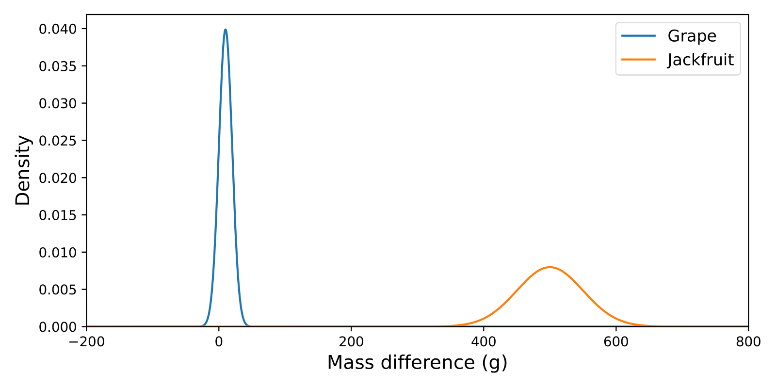
Consider the situation where we want to predict the mass of fruit (as in the figure below). Given the conformal predictors of the previous section, we can already get somewhere.
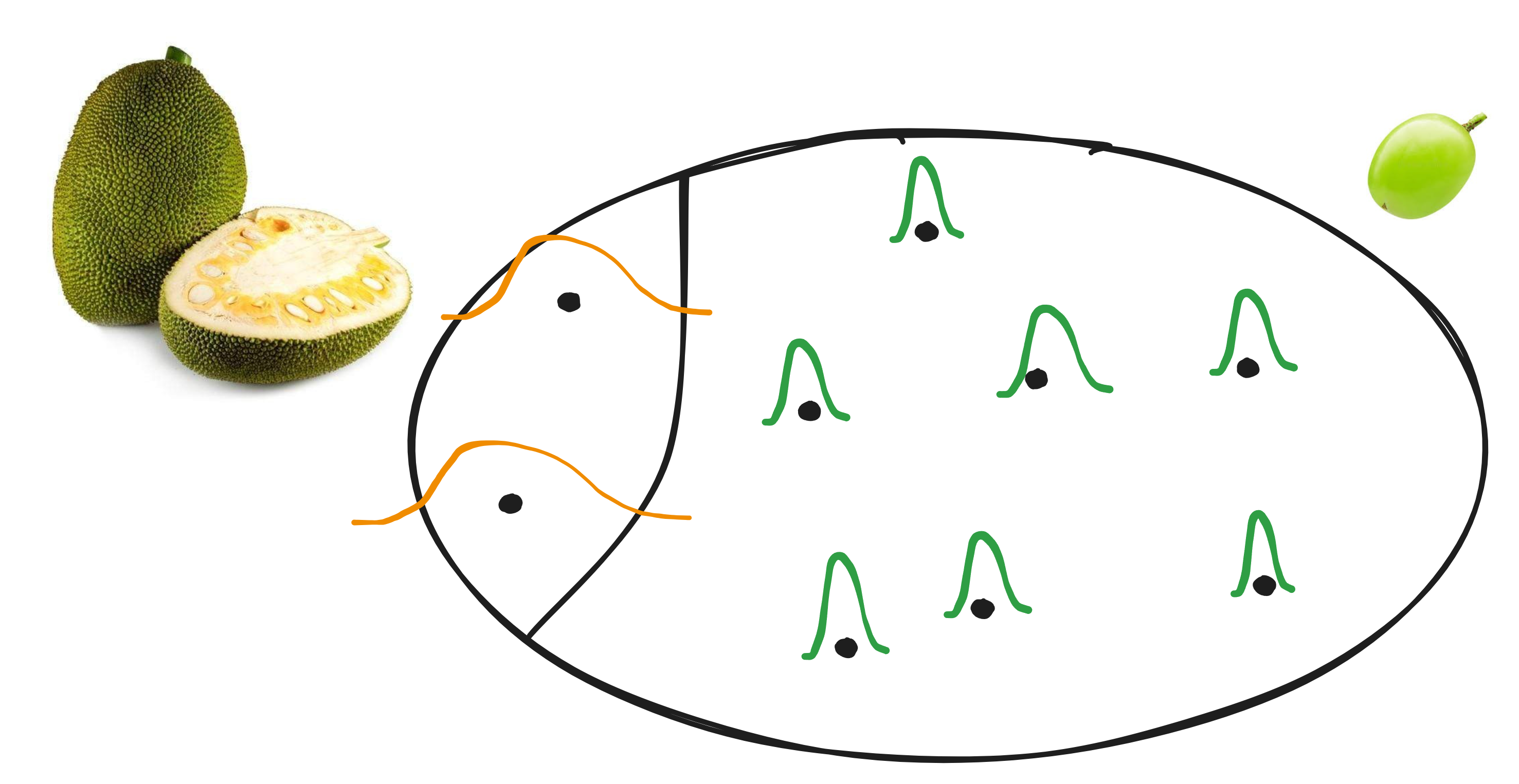
However, when our population of fruits contains very different types of fruit (grapes and jackfruit in our case), the marginal validity results might lead to unexpected behaviour. If the majority of our fruit consisted of grapes and the model had residuals as shown in the graph below, we might produce reasonable prediction intervals for grapes, but the intervals for jackfruit will be much too small.
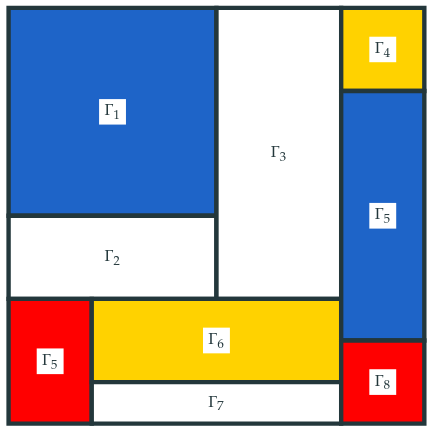
For a solution, here, we are inspired by the painter Mondriaan. Instead of constructing one overall conformal predictor, we first split the instance space $\mathcal{X}\times\mathcal{Y}$ and construct a separate model for every block.
The downside with this approach is, however, that we need enough calibration data for every block in the partition. So, the question I asked myself is: “When can a single conformal predictor approximate conditional validity?”. This led us to a more classical notion from parametric statistics.
A classic example would be standardization as shown below.
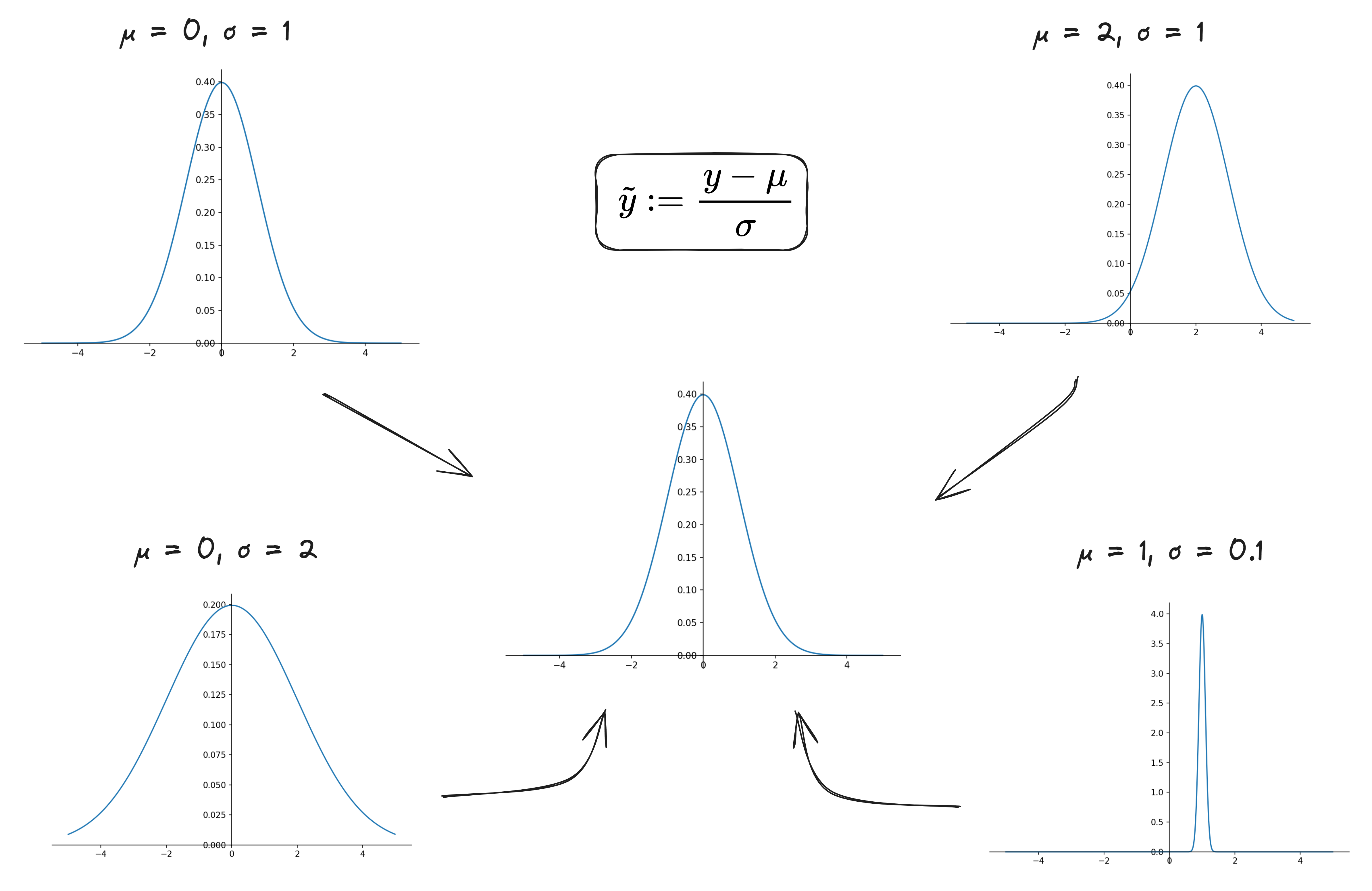
Armed with this idea, we came to the following contribution.
The underlying idea is simply that when the distributions for each class match, we can simply throw all data together. Returning to the case of standardization and the standardized nonconformity measure introduced on the previous section, the following corollary holds.
Comparing the two preceding sections, we have the following scenario:
- Mondrian approach: strong guarantees, but data required per class.
- non-Mondrian approach: guarantees (in pivotal scenario) but data required for accurate models.
The result is that, in settings with limited data, a strictly conditional approach might not work. To this end, we consider something in between marginal and conditional validity.
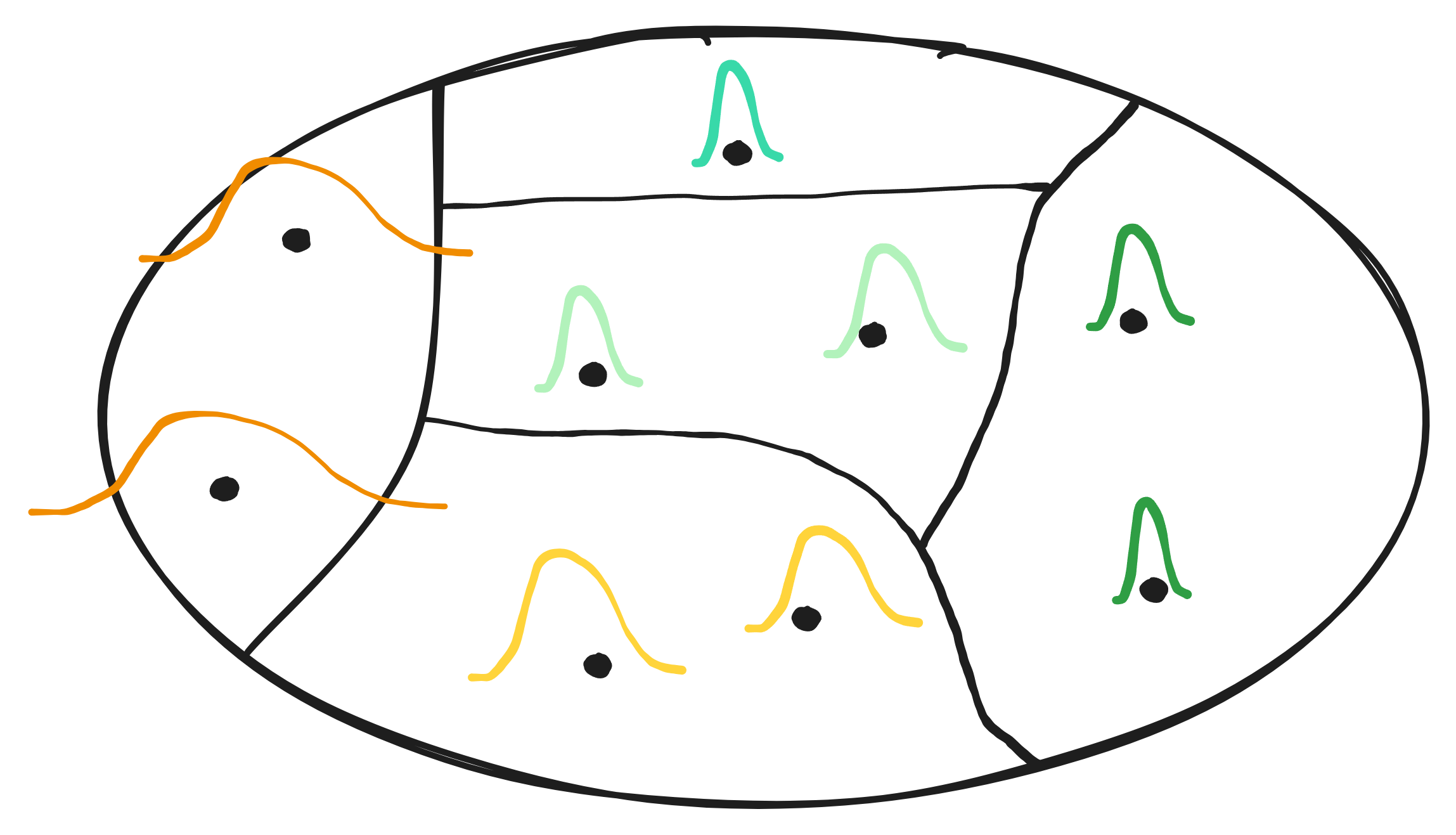
In the figure below, we can see that the data distributions differ between the different groups. However, taking into account the colours, some groups are more similar than others. This is the main idea of clusterwise validity. We will group ‘similar’ classes, achieving strict validity on each group due to the Mondrian approach, but still approximating conditional validity as well as possible.
Because this approach is rather recent, there were still some important gaps in the literature. For example, the statement above, although general, only talks about the Mondrian structure, which can be rather complex and is often not determined by clustering methods4. However, to group together similar data points, data-driven clustering methods are very popular. Our idea was then to find out how clustering nonconformity scores could be related to clustering inputs.
This led to the following contribution.
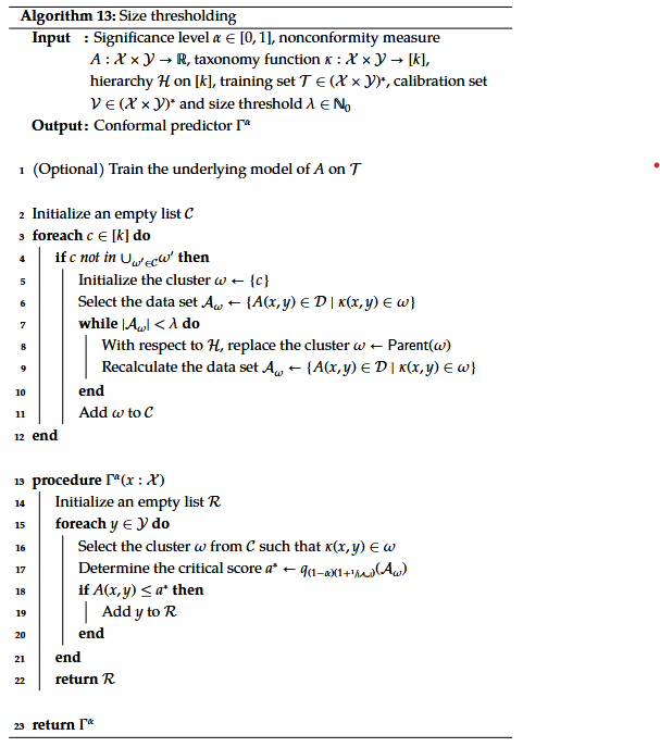
Besides this theoretical contribution, we also looked at a more practical problem. What happens in the case of extreme classification, i.e. classification problems with a large number of classes (e.g. thousands or more). In such cases, it is often impossible to have enough calibration data for every class. Here we looked at an ‘informed’ approach, where side information could be included. In our case, the side information was presented in the form of a class hierarchy. Such a hierarchy leads to a natural clustering of the classes. In fact, a multilayer hierarchy induces many different clusterings and, as such, allows us to use an adaptive strategy. Given a (cluster) size threshold $\lambda\in\mathbb{N}$, we can use the finest clustering such that every cluster contains at least $\lambda$ data points. This algorithm is presented in pseudocode below:
A natural example of hierarchies is found in biology. For example:

After a journey of four years, the story is, of course, not over. Many important and/or interesting questions remain. Some that I would have liked to answer or, at least, see answered in the upcoming years are:
- How can contexts/side information be better incorporated into conformal prediction? (E.g. through novel nonconformity measures, through the design of better, possibly adaptive Mondrian taxonomies, …)
- How can conformal prediction be used in the general study of uncertainty quantification (epistemic vs. aleatoric uncertainty, etc.) and vice versa?
- Can conformal predictors be composed in a sensible way (in the sense of Fong and Spivak5), e.g. do they admit functional composites or (tensor) products?
- T. Gneiting, & A. E. Raftery. (2007). Strictly proper scoring rules, prediction, and estimation. Journal of the American statistical Association, 102(477), 359–378.
-
We will not go into full detail of what uncertainty could encompass. This very interesting, but also very complex scientific and philosophical question will be left aside. ↩
-
Unless extensions are considered (e.g. those incorporating sequential dependence such as for time series modelling). ↩
-
For stability, the model predicts the logarithm of the variance. ↩
-
Mondrian taxonomies are often constructed by hand based on domain knowledge. ↩
-
See “An Invitation to Applied Category Theory: Seven Sketches in Compositionality” by Fong and Spivak (2019). ↩