Normalizing flows for regression problems
This talk, given as part of the Machine Learning Discussion Group of KERMIT, had three goals:
- Giving an introduction to the formal (measure-theoretic) foundations of probability theory.
- Explaining how to transform an arbitrary distribution into a normal distribution.
- Applying the normalizing flow framework to regression problems.
The structure of the talk was as follows:
- Short introduction on measure theory,
- Introduction to flows,
- How flows can be applied to regression problems, and
- Some extras on ODEs.
For a refresher (or introduction) on measure theory, see the appendix. The most important concept for this post is that of a measure. For the study of (normalizing) flows, it is important to consider the convergence of measures. A sequence of measures $(\mu_n)_{n\in\mathbb{N}}$ on a measurable space $(\mathcal{X},\Sigma_{\mathcal{X}})$ is said to converge weakly to a measure $\mu$ if
\[\lim_{n\rightarrow\infty}\int_\mathcal{X}g\,d\mu_n=\int_\mathcal{X}g\,d\mu\]for all bounded, continuous functions $g:\mathcal{X}\rightarrow\mathbb{R}$. Note that for probability measures, this simply means that the expectations converge. (This explains why this is a weak form of convergence.) Now, because of the theorem above, if a sequence of measurable functions $(f_n)_{n\in\mathbb{N}}$ converges pointwise to a function $f:\mathcal{X}\rightarrow\mathcal{Y}$, the pushforwards converge weakly:
\[\forall x\in\mathcal{X}:\lim_{n\rightarrow\infty}f_n(x)=f(x)\implies f_{n,\ast}\mu\rightsquigarrow f_\ast\mu\,.\]A flow is a continuous function $\phi:\mathbb{R}\times\mathcal{X}\rightarrow\mathcal{X}:(t,x)\mapsto\phi_t(x)$ satisfying:
- $\phi_0=𝟙_\mathcal{X}$,
- $\phi_t\circ\phi_s=\phi_{t+s}$ for all $s,t\in\mathbb{R}$, and (as a consequence)
- $\phi_t$ is invertible for all $t\in\mathbb{R}$ with $\phi_{-t}=(\phi_t)^{-1}$.
In practice, this is often approximated by a “discrete flow” $\phi:\mathbb{Z}\times\mathcal{X}\rightarrow\mathcal{X}$:
\[\phi_k:=\Phi^k\]for some transformation $\phi_1\equiv\Phi:\mathcal{X}\rightarrow\mathcal{X}$ (the time-1 map of the continuous flow). As a further approximation, we can replace the iterated power structure by an arbitrary sequence of transformations:
\[\Psi:=\Phi_k\circ\ldots\Phi_2\circ\Phi_1\,,\]with all $\Phi_i$ invertible. If all these transformations are diffeomorphisms, the change-of-variables formula becomes:
\[f_X(x) = f_{\Psi(X)}\bigl(\Psi(x)\bigr)\prod_{i=1}^k\left|\frac{\partial\Phi_i}{\partial\Phi_{i-1}}\bigl(\Phi_{i-1}(x)\bigr)\right|\,.\]The most common transformations are the following ones (here it is assumed that $\mathcal{X}$ is a vector space):
- Affine (or linear) flow: $\Phi(x) := Ax+b$.
- Planar flows: $\Phi(x) := x + h(w\cdot x + \lambda)v$ for some diffeomorphism $h:\mathbb{R}\rightarrow\mathbb{R}$.
- Coupling flows: $\Phi(x) := \bigl(x^I,h(x^J;x^I)\bigr)$ for some diffeomorphism $h:\mathbb{R}^{|J|}\times\mathbb{R}^{|I|}\rightarrow\mathbb{R}^{|J|}$, where $x=(x^I,x^J)$ for some partition $I,J$ of $\{1,\ldots,\dim(\mathcal{X})\}$.
Although not very expressive, e.g. exponential families are mapped to exponential families, affine flows are simple to implement. By contrast, the planar flows are expressive, but their inverse generally does not exist in closed form.
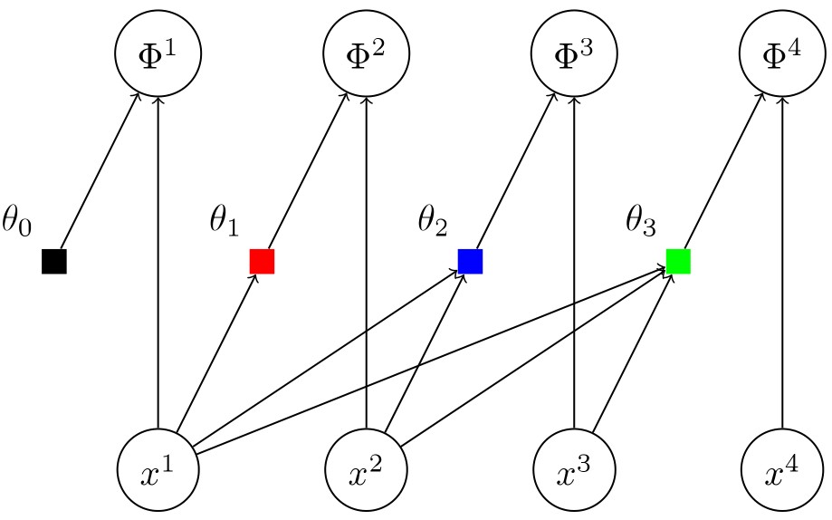
The most powerful transformation is the so-called autoregressive (or triangular) flow. In components it is given by
\[\Phi^\mu(x) := h_\mu\bigl(x^\mu;\theta_\mu(x^1,\ldots,x^{\mu-1})\bigr).\]The structure of such a flow is shown in the figure below.

The reason for why autoregressive flows are so important is given by the following theorem which implies the universality of the classes of autoregressive flows with increasing coupling functions (or any dense subset thereof) for distributions without discrete or singular contributions:
To obtain a normalizing flow (on $\mathbb{R}^d$), we now make the following crucial assumption:
\[\Psi(X)\sim\mathcal{N}(0,𝟙_{d\times d})\,.\](We could essentially use any fixed distribution, but normal distributions are much easier to work with.) To generate new samples, we simply sample points from a multinormal distribution and pass them through the flow function.
As mentioned at the end of the previous section, for generative models the joint distribution of, for example, the pixels of a picture is transformed to a (multi)normal distribution:
\[\Psi:P(X)\Rightarrow\mathcal{N}\,.\]However, for regression problems it is not the joint distribution that is transformed. It is the conditional distribution $Y\mid X$ that should be transformed.
This is achieved by making the flow parameters $\mathcal{X}$-dependent: \(\Psi_X:P(Y\mid X)\Rightarrow\mathcal{N}.\)
This means that instead of directly optimizing the flow parameters, we train a network that outputs these parameters given the features.
In theory, for univariate absolutely continuous CDFs the following transformation suffices: $\Psi := G^{-1}\circ F$. This first maps $F$ to the uniform distribution on $[0,1]$ and then, with the quantile function, the uniform distribution is mapped to $G$. However, this requires the knowledge of both $F$ and $G^{-1}$ (in closed form if we want to implement this). Since this is not possible, we replace the transformation by a sequence of simpler ones and apply variational optimization using the loglikelihood
\[\mathcal{L}(\mathcal{D}) = \sum_{(\mathbf{x},y)\in\mathcal{D}}\left(\log\Bigl(\mathcal{N}\bigl(\Psi(y\mid\mathbf{x})\bigr)\!\Bigr) + \sum_{i=1}^k\log\dot{\Phi}_i\bigl(\Phi_{i-1}(y\mid\mathbf{x})\bigr)\!\right)\,,\]where:
- $\Psi(\,\cdot\mid X):\mathbb{R}\rightarrow\mathbb{R}$ is the total transformation $P(Y\mid X)\rightarrow\mathcal{N}$.
- Each $\Phi_i$ is modeled by a monotone network: \[\Phi_i(y\mid\mathbf{x}) := \int_0^y\bigl(f_i(u,\mathbf{x})+1\bigr)\,\mathrm{d}u + \text{cnst}\] with $f_i:\mathbb{R}\times\mathcal{X}\rightarrow\mathbb{R}$ an unconstrained neural network with final ELU activation.
Instead of discretizing the flow $\phi:\mathbb{R}\times\mathbb{R}^d\rightarrow\mathbb{R}^d$, we can use the fact that flows are usually the solutions of an ordinary differential equation (ODE). For example, consider
\[\Phi_{(k)}:=\mathbb{1}_{d\times d} + \tfrac{1}{k}\xi\qquad\text{with}\qquad\xi\in M_d(\mathbb{R})\,.\]The powers $\Phi_{(k)}^k$ converge to the exponential map $\exp(\xi)$, which is the (time-1 map of the) solution of the ODE
\[\dot{x}(t) = \xi\triangleright x(t)\,,\]where $\triangleright$ indicates the action of $M_d(\mathbb{R})$ on $\mathbb{R}^d$. This observation leads to modelling normalizing flows as neural ODEs. Another approach is to model the flows using stochastic differential equations instead of ODEs. For a vanishing diffusion term, this recovers the ODE approach.
The goal of training NFs is to find a measurable function $\Psi$ such that $\Psi_\ast P=\mathcal{N}$, where $P$ is the data generating distribution. This problem is actually the same as the one considered in optimal transport:
\[\text{minimize }\int_\mathcal{X}c\bigl(x,\Psi(x)\bigr)\,\mathrm{d}\mu(x)\qquad\text{with}\qquad\Psi_\ast\mu=\nu\,.\]Here, the challenge is to find the minimal cost for transporting products from producers, distributed according to $\mu$, to consumers, distributed according to $\nu$.
- Kobyzev, I., Prince, S. J., & Brubaker, M. A. (2020). Normalizing flows: An introduction and review of current methods. IEEE transactions on pattern analysis and machine intelligence, 43(11), 3964-3979.
- Bogachev, V. I., Kolesnikov, A. V., & Medvedev, K. V. (2005). Triangular transformations of measures. Sbornik: Mathematics, 196(3), 309-335.