
Pictorial Bayes
This post contains the content of a talk, titled “Drawing pictures with Nico”, that I gave for the Statistics Discussion Group at the Faculty of Bioscience Engineering (UGent). I have reworked parts of the talk and elaborated on many concepts. Moreover, I have added an ‘optional’ part at the end which puts everything within a much more abstract setting.
The structure of the talk was as follows:
- Short introduction on probability theory,
- Diagrammatic methods for Markov categories,
- Rigidity for finite sets,
- Contexts as categories, and
- Geometric ideas for higher mathematics.
In most (applied) courses on probability theory and statistics, the definition of a probability distribution is given for either the case of finite sets or Euclidean spaces, without explicitly referencing the underlying structure. Moreover, many subtleties and possible problems are ignored. For a more complete introduction, see the appendix on measure theory.
The first part of the talk consisted of a formal treatment by first considering the notion of event, and only then, introducing the collection of distributions compatible with these events. For an arbitrary set $\mathcal{X}$, a good choice of events, called measurable subsets, is given by the notion of $\sigma$-algebras.
There exist two trivial examples:
- The trivial $\sigma$-algebra: $\Sigma_\text{trivial}:=\{\emptyset,\mathcal{X}\}$, and
- The discrete $\sigma$-algebra: $\Sigma_\text{disc}:=2^\mathcal{X}$.
The latter is, for example, the one used in the definition of discrete distributions. Note that these collections can be defined on any set, they do not use any structure on $\mathcal{X}$. On these $\sigma$-algebras, we can then define the notion of (probability) measure (or distribution). An important probability measure for this talk is the Dirac measure:
\[\delta_x(A) := \mathbb{1}_A(x) = \begin{cases} 0&\text{if }x\not\in A\,,\\ 1&\text{if }x\in A\,. \end{cases}\]As with most mathematical structures, we like to consider functions that preserve the given structure. For measurable spaces, the correct notion is that of a measurable function. The reason for using the preimage has to do with the definition of events. Disjoint unions are not preserved under (direct) images.
- For every $A\in\Sigma_\mathcal{Y}$: $x\mapsto f(A\mid x)$ is measurable.
- For every $x\in\mathcal{X}$: $A\mapsto f(A\mid x)$ is a probability measure.
Some examples of kernels are:
- Random walk: $p(i\mid j) := p\delta_{i,j+1} + (1-p)\delta_{i,j-1}$

- Identity function: $\mathbb{1}(i\mid j) := \delta_{i,j}$

- Measurable function: $f(i\mid j) := \delta_{i,f(j)}$
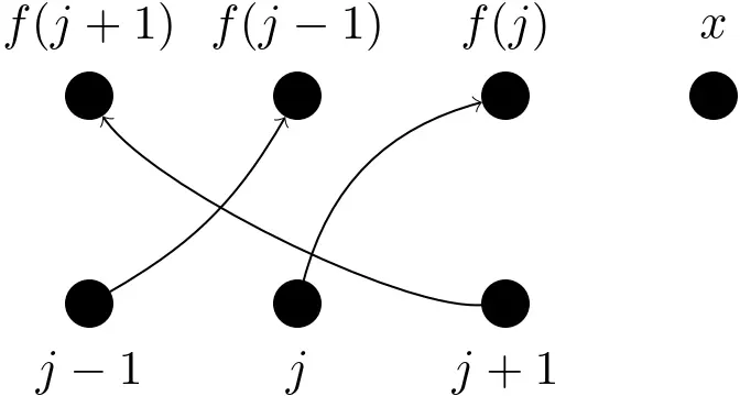
Integration (against a probability measure) will not be introduced in detail (even though it was necessary for this talk). Suffice it to say that it reduces to summation in the case of point masses (and discrete distributions) and to ordinary (Riemann) integrals in the case of density functions.
The basic ingredients of any diagram are lines (or arrows):

The convention in this post is that diagrams have to be read from left to right. The interpretation of arrows depends on the context:
- Set theory: functions $X\rightarrow Y$,
- Linear algebra: linear maps $X\rightarrow Y$, or
- Probability theory: Markov kernels $X\rightarrow\mathbb{P}(Y)$.
Probability measures, also called states in this setting, are arrows out of the one-element set $\mathbf{I}:=\{\ast\}$:

Joint states are simply indicated by multiple outgoing lines:

Given the above information, the context for a diagrammatic calculus can be fixed. The following notations will be used in the remainder:
- Set: Sets and ordinary functions,
- Vect (technically FinVect): (Finite-dimensional) vector spaces and linear maps,
- Meas: Measurable spaces and measurable functions,
- $\mathbf{Stoch}$: Probability spaces and Markov kernels,
- $\mathbf{BorelStoch}$: Borel probability spaces and Markov kernels, or
- $\mathbf{FinStoch}$: Finite probability spaces and Markov Kernels.
Concatenation of lines or arrows is, in general, given by a suitable notion of composition:

The interpretation, again, depends on the context:
- Set, Vect & Meas: function composition $g\circ f$, or
- $\mathbf{Stoch}$: Chapman–Kolmogorov equation \[(g\circ f)(A\mid x) :=\int_\mathcal{Y}g(A\mid y)\,df(y\mid x)\,.\]
Lines or arrows can also be combined in different ways:
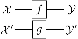
- Parallel functions: $f\otimes g:\mathcal{X}\otimes\mathcal{X}’\rightarrow\mathcal{Y}’\otimes\mathcal{Y}’$
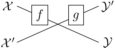
- ‘Braided’ functions: $x\otimes x’\mapsto g(x’)\otimes f(x)$
Every measurable space $(\mathcal{X},\Sigma_{\mathcal{X}})$ admits two `structure morphisms’:
- The deletion map: $\mathrm{del}_\mathcal{X}(x) := 1$

which corresponds to integrating out a variable: $\displaystyle\int_\mathcal{Y}df(y\mid x)$

- The copy map: $\mathrm{copy}_\mathcal{X}(A\times B\mid x) := \delta_x(A)\delta_x(B)$
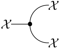
which corresponds to transporting a distribution on $\mathcal{X}$ to one on its diagonal embedding in $\mathcal{X}\otimes\mathcal{X}$.
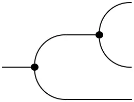
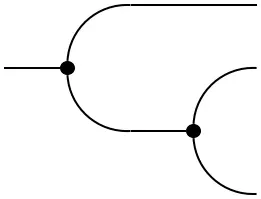
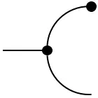
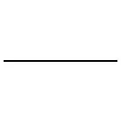
These morphisms endow a probability space with the structure of an (internal) comonoid:
 =
=
and
 =
=
 =
=
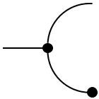
The idea behind comonoids can be understood by turning these diagrams around (i.e. ‘inverting time’). The first equation is then simply the associativity of a multiplication map and the second equation is the unit law. (Sets with a multiplication map with these properties are also called monoids.) Such ‘dual’ definitions are a common occurrence in abstract parts of mathematics. It is a nice intuition to have!
Probability spaces are even (co)commutative comonoids:
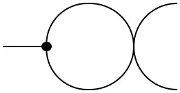 =
=
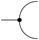
More generally, contexts $\mathbf{C}$ where the structure morphisms $\mathrm{del}$ and $\mathrm{copy}$ exist and satisfy the (co)commutative comonoid conditions are called Markov categories or copy-discard (CD) categories.
Every set admits a unique comonoid structure with respect to the Cartesian product (which can also be thought of as a tensor product for which the unit is the one-element set $\mathbf{I}$):
- Delete morphism: unique function to $\mathbf{I}$.
- Copy morphism: diagonal embedding $x\mapsto(x,x)$. Vector spaces do not admit this diagonal comonoid structure. Can you see why? (In physics, this gives rise to the no-cloning theorem!)
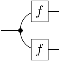
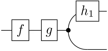
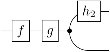
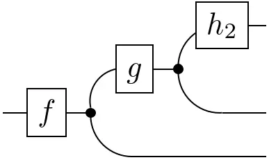
Using the above diagrammatic rules, various notions from probability theory can be represented. Some examples will be covered below.
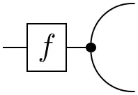 =
=
 =
=
 =
=
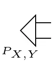 =
=
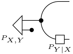
When working with states (or functions) of higher arity, e.g. a joint state on three variables, conditioning can be done in different ways. By 'simple' diagrammatic manipulations, the following property can be proven whenever $\mathbf{C}$ has all conditionals:
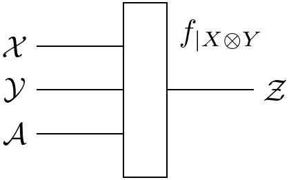 =
=
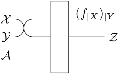
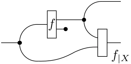
Note that the definition of conditionals is not reserved to states $\mathbf{I}\rightarrow\mathcal{X}\otimes\mathcal{Y}$. It can be generalized to arbitrary functions $\mathcal{Z}\rightarrow\mathcal{X}\otimes\mathcal{Y}$:
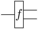 =
=
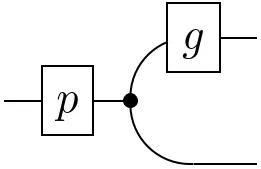
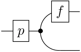 =
=
From here on, attention will be restricted to finite sets, i.e. we work in $\mathbf{FinStoch}$ (unless stated otherwise). These will be equipped with the discrete $\sigma$-algebra. In this case, (probability) measures are defined by their values at points and can be written as vectors. Moreover, kernels can be expressed as matrices. To allow for some more diagrammatic freedom, functions are generalized from Markov kernels to transition kernels, where the latter need only take values in the set of measures (which can be unnormalized).
Every object $(\mathcal{X},\Sigma_{\mathcal{X}})$ admits the structure of an (internal) monoid:
- Unit map: $\varepsilon_\mathcal{X}(x) := 1$

- Multiplication map: $\mu_\mathcal{X}(x\mid i,j) := \delta_{i,x}\delta_{j,x}$
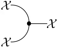
As before, this structure is commutative with respect to the (trivial) braiding. As noted in the previous section, the definition of a comonoid was dual to that of a monoid. This is clear when comparing the explicit formulas for the comultiplication and counit to the expressions above. The multiplication $\mu$ and unit $\varepsilon$, consequently, also satisfy the associativity condition and unit law. Finite probability space not only carry the structure of a monoid and comonoid, they are even compatible in an elegant way. Such objects are called Frobenius monoids:
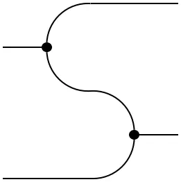 =
=
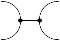 =
=
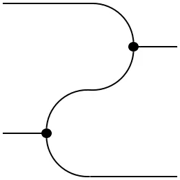
 =
=
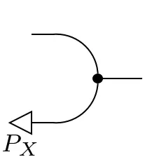
 =
=

 =
=
 =
=

Using the different structures on a finite probability space $(\mathcal{X},\Sigma_{\mathcal{X}})$, even more diagrammatic objects can be obtained:
- Cups:
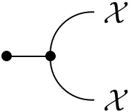 =
$\mathrm{coev}_\mathcal{X}(x,x') = \delta_{x,x'}$
- Caps:
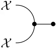 =
$\mathrm{ev}_\mathcal{X}(x,x') = \delta_{x,x'}$
The cup and cap give rise to a so-called rigid structure (see further below) because they satisfy the triangle identities or yanking conditions:
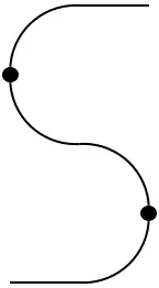 =
=
 =
=
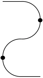
The reason for the term ‘yanking condition’ stems from the fact that the bends in the lines can be ‘yanked out’.
Although the diagonal comultiplication does not exist for vector spaces, a rigid structure exists on finite-dimensional vector spaces. For a vector space $V$, choose a basis $\{e_i\}_{i\leq\dim(V)}$ and denote its dual basis by $\{e^i\}_{i\leq\dim(V)}$.
- Cup: $\mathrm{coev}_V(\lambda) := \sum_{i=1}^{\dim(V)}\lambda e^i\otimes e_i$.
- Cap: $\mathrm{ev}_V(e_j\otimes e^i) := e^i(e_j) = \delta^i_j$.
As an example of diagrammatic calculus, the ‘bubble diagram’ gives the dimension of the vector space (more generally, the trace of a linear map):
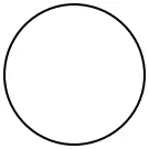 =
$\sum_{i=1}^{\dim(V)} e^i(e_i) = \sum_{i=1}^{\dim(V)}\delta^i_i = \dim(V)\,.$
These constructions, and their extensions to superspaces, are also of importance in theoretical physics! (I might write more about this in a future post.)
Using the cup and cap, we can also express the transposition of linear maps:
 =
=
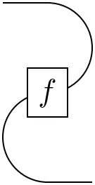
Again, the proof is left as an exercise to the reader. It can easily be obtained using the expressions introduced above ;-)
The cups and caps of finite probability spaces can be altered using the (inverse) modifiers:
 =
=
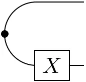
and
 =
=
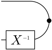
With the modified caps, the conditionals can be given a more explicit expression, which closely resembles the equational definition:
 =
=
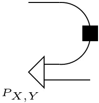
In the context of linear algebra, it was shown how the cups and caps allow us to express transposition by bending lines around. Using the modified cups and caps, transposition of a conditional in $\mathbf{FinStoch}$ gives Bayes’ theorem:
 =
=
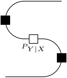
The previous sections should have given an idea of how diagrammatic tools can be used to study vastly different areas of mathematics and science. The reason that this is possible is not a mere coincidence. What were called ‘contexts’ and, more specifically, the specific contexts that were considered, all share the same structure. This section aims to introduce the terminology used to describe these structures.
- Objects: $\mathrm{ob}(\mathbf{C})$, and
- Morphisms: $\mathrm{hom}(\textbf{C})$.
These should satisfy the following conditions:
- Identity: For all $X\in\mathrm{ob}(\mathbf{C})$, there exists an identity morphism $\mathbb{1}_X\in\mathbf{C}(X,X)$.
- Associativity: $f\circ(g\circ h) = (f\circ g)\circ h$, whenever the compositions are well-defined.
Some examples were already given after the introduction of ‘lines’. Some more exotic examples are (the first 2/3 are a good exercise for drawing diagrams):
- Every poset (partially ordered set) is a category, where a unique morphism $x\rightarrow y$ exists whenever $x\leq y$.
- Every directed graph defines a category. (The free category generated by that graph.)
- The category Cat of small categories, i.e. those where $\mathrm{ob}(\mathbf{C})$ and $\mathrm{hom}(\mathbf{C})$ are sets. (The morphisms are defined below.)
- The representations of a (finite) group with intertwiners (equivariant functions) as morphisms.
Just as there are functions between sets, there are also operations between categories.
- $F$ maps objects $X$ to objects $FX$.
- $F$ maps morphisms $X\rightarrow Y$ to morphisms $FX\rightarrow FY$.
- $F$ preserves composition.
The Giry monad that assigns probability measures to measurable spaces was the first example of a functor. Some other examples are:
- The power set functor $P:\textbf{Set}\rightarrow\textbf{Set}$, which assigns power sets and (pre)images.
- The Yoneda embedding of an object $X\in\mathrm{ob}(\mathbf{C})$, which assigns to every other object $Y\in\mathrm{ob}(\mathbf{C})$ the morphisms $\mathbf{C}(Y,X)$. Morphisms $f$ are mapped to precompositions $-\circ f$.
The second example is one of the most foundational constructions in category theory!
We can also define morphisms $\kappa:F\Rightarrow G$ between functors.
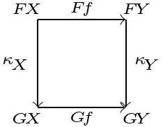
Some (technical) examples are (some other examples will pop up in the next few sections):
- The identity natural transformation $F\Rightarrow F$.
- Double duals: there exists a natural transformation $\eta_{V}:V\rightarrow V^{**}$ for finite-dimensional vector spaces. (For the single dual $V\rightarrow V^*$, the transformation is ‘unnatural’ since it requires a choice of basis.)
- For any morphism $f:X\rightarrow Y$ there exists a natural transformation between the Yoneda embeddings of $X$ and $Y$. This is given by postcomposition $f\circ -$.
Whereas objects are represented by vertices and morphisms by lines in a diagrammatic calculus, natural transformations could be represented by filling in the area between two parallel functors (parallel here means that they have the same domain and codomain). This extension of diagrams to higher-dimensional structures will play a role at the end of this talk.
To express parallel objects and morphisms, the structure of a tensor product needs to exist.
- Associativity: $X\otimes(Y\otimes Z)=(X\otimes Y)\otimes Z$\pause, and
- Unit: $X\otimes\mathbf{I}=X=\mathbf{I}\otimes X$.
In some monoidal categories, the tensor product is symmetric in a certain sense.
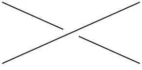 =
=
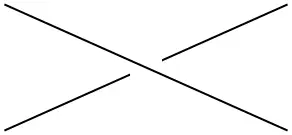 =
=
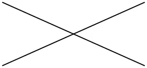
For cups and caps, another structure is required.
It is time to relate the categorical notions to the sections on probability theory. Only one piece of data is still missing.
Putting everything together gives the central object of ‘categorical probability theory’.
To model morphisms such as Markov kernels, some more structure is needed.
- Objects: $\mathrm{ob}\bigl(\mathrm{Kl}(T)\bigr):=\mathrm{ob}(\mathbf{C})$, and
- Morphisms: $\hom_{\mathrm{Kl}(T)}(X,Y):=\hom_{\mathbf{C}}(X,TY)$.
All this data probably looks rather scary and technical (it is). However, it is more useful than it might appear. Many effects in computer science can be modelled using monads and Kleisli morphisms. Almost any process with ‘side effects’ such as I/O operations can be modelled using a monad. (People that use Haskell love this stuff.)
If $\mathbf{C}$ is a Markov category and $T:\mathbf{C}\rightarrow\mathbf{C}$ is a monad that preserves the product and unit, $\mathrm{Kl}(T)$ is again a Markov category. Moreover, on any Cartesian monoidal category, i.e. a category where the monoidal structure is given by the Cartesian product such as in $\mathbf{Set}$, every object has a unique comonoid structure (diagonal embedding $\mu:x\mapsto x\times x$). The Giry monad $\mathbb{P}$ preserves this structure and, hence, induces a Kleisli category $\mathrm{Kl}(\mathbb{P})$ that is Markov. This is exactly the category $\mathbf{Stoch}$ of Markov kernels from before (hence the name).
(Small) Categories can be built up geometrically from triangles. This follows from the fact that for any two composable morphisms, we obtain the following diagram
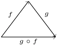
By pasting all these triangles along shared edges, (small) categories can be represented as simplicial complexes. (A simplex is a higher-dimensional generalization of a triangle.) If instead of being exactly equal, composition is only defined up to some higher-dimensional morphisms, a 2-morphism, the notion of quasicategory is obtained. This corresponds to filling in the triangles:
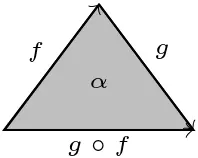
In a similar way, we could fill in pyramids (3-simplices) by 3-morphisms and so on.
- Capiński, Marek, and Peter E. Kopp. (2004). Measure, integral and probability. Vol. 14. Springer.
- Fritz, Tobias. (2020). A synthetic approach to Markov kernels, conditional independence and theorems on sufficient statistics. Advances in Mathematics 370: 107239.
- Coecke, Bob, and Robert W. Spekkens. (2012). Picturing classical and quantum Bayesian inference. Synthese 186: 651–696.
- $n$Lab